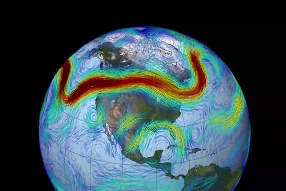
Jet streams occur in the upper troposphere at locations where warmer air mass is separated from cooler air mass. They are formed at these boundaries by rising warm air and sinking cooler air, under the action of the Coriolis force, which redirects the vertical motion eastward (more on this later.) Two dominant jet streams in the northern hemisphere are the Polar Jet (9 to 12 kilometers altitude, typically at 50 to 60 degrees latitude) and the Subtropical Jet (10 to 16 kilometers altitude, typically at 30 degrees latitude). Corresponding jet streams occur in the southern hemisphere. The actual jet streams form very wavy tracks, and their mean latitude moves southward during summer and northward during winter, as illustrated in Figure 1.
The jet stream cross section is typically a few hundred kilometers horizontally and about 5 kilometers vertically, with wind speeds from 100 to 200 kilometers/hour. Underneath the jet stream, winds follow the same track but with decreasing speed with decreasing altitude as illustrated below in Figure 2. They are one of the more influential factors in surface weather patterns.
Generation of Jet Streams
Global wind patterns are driven by a combination of thermal and gravitational forces. In a hydrostatically stable atmosphere, the gravitational force is balanced against the gradient in the pressure. When there is variation in surface temperature, the air in warmer regions expands and rises, then flows at upper altitude toward regions that are cooler. The air then cools, contracts, and sinks toward the surface. The cooler surface air then completes the circulation by flowing back toward the warm region at the lower altitude.
In place of one large circulation between the warm equator and the cool polar region, the actual global pattern has three such circulations: the Hadley, Ferrel, and Polar Cells. Figure 3 below presents a meridian (north-south) cross section of these circulations. Note that the height of the Tropopause decreases moving from the equator toward the pole. At the surface, low pressure bands occur at the equator and at the boundary between the Ferrel and Polar Cells, where the air is rising. High pressure bands occur at the boundary between the Hadley and Ferrel Cells and at the pole, where the air is sinking. High pressure is associated with fair and dry/hot weather. Low pressure is associated with rainy and stormy weather.
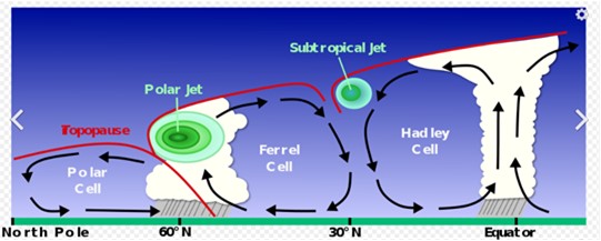
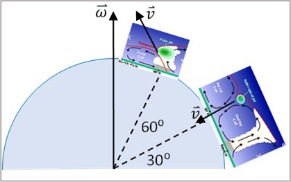
Figure 3 also shows the two jet streams. They both flow eastward (into the page) and are caused by the Coriolis force acting on the upper air motion of the global circulation cells. In a rotating frame of reference – like the rotating Earth – the Coriolis force turns a moving mass to the right in the northern hemisphere and to the left in the southern hemisphere. The force vector, F, on a unit of the atmosphere with a mass, m, is expressed mathematically as a cross product between the Earth rotation axis vector, w, and the mass velocity vector, n:
F = -2m w X n
Note that the force acts on any moving mass unless it is moving parallel to the axis. Another way to understand it, from an inertial frame of reference, is that the air mass has angular momentum as it rotates with the Earth. If air moves toward the Earth’s axis, it must increase its eastward speed to conserve the angular momentum. These explanations would seem to be consistent with the Subtropical Jet in Figure 3, but not for the Polar Jet. The problem is in the flat-Earth view. If we reorient the circulations at the jet stream locations in a curved-Earth view, as in Figure 4, we see that both explanations (Coriolis force formula and the conservation of angular momentum) lead to an eastward flow.
Hurricane Hunter Satellite Measurement and Characterization of Jet Streams
Figures 3 and 4 also indicate the likelihood of large cumulus clouds due to the upward air flow along the Polar Vortex. This raises the possibility of tracking the Polar Jet stream directly from cloud formations viewed from space. Figure 5 presents side-by-side views of a jet stream forecast (left) and a corresponding Earth/cloud visible image from space (right). The NetWeather jet stream forecast is based on a combination of atmospheric measurements and modeling; the NASA Worldview is a daily assembly of over 1,000 full-resolution satellite imagery layers from the Earth Observing System Data and Information (EOSDIS) program. The jet stream corresponding to the forecast appears to be clearly visible in the image on the right. The red square overlaid on the image represents the extent of a single stereo data collect from one overpass of a pair of TWA’s Hurricane Hunter Satellites.
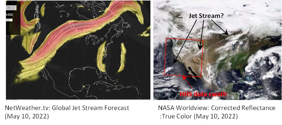
This would provide hundreds of thousands of 3D wind data points with 300 to 500 meters spatial footprint as well as ±100 meters geolocation and altitude accuracy, and 1 meter/second wind vector accuracy (see “Hurricane Hunter Satellites”]. This combination of geographic coverage and measurement accuracy in 3D will enable unprecedented characterization of the dynamic structure of the jet stream along its length.
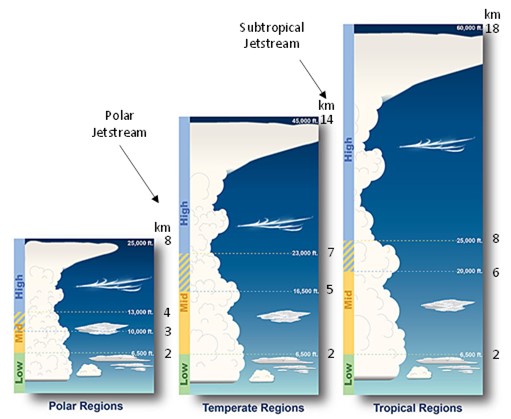
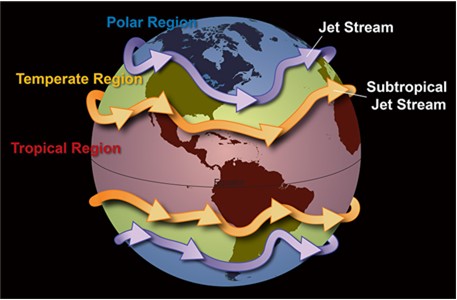
When the cumulus clouds associated with the jet streams are not clearly present in the visible images, we may still be able to roughly locate the jet streams by taking advantage of the abrupt change in the height of the troposphere at the jet stream location and the associated change in characteristic height of various cloud types on either side of the jet stream. Figure 6 presents the characteristic height of four basic cloud types in the three geographic zones separated by the jet streams: the Polar Jet is bounded by the Polar and Temperature Regions, and the Subtropical Jet is bounded by the Temperate and Tropical Regions. The lowest characteristic cloud heights (cumulo-form and strato-form) do not change from one zone to the next, but the mid-level clouds (mostly Strato-form) and especially the high-level clouds (cirro-form and the giant nimbo-form) change characteristic height enough to serve as a diagnostic of the region (Polar, Temperate, or Tropical). With the widespread and accurate determination of cloud heights over a typical HHS data collect area of 2,000 x 2,000 kilometers, we should be able to identify the approximate geographic location of the boundaries of these regions that are associated with the jet streams.
